Entropy and cross-entropy loss

Entropy and cross-entropy

Entropy

\[H(X) = -\sum p_i log_2 pi\] \(p_i\) is the proportion of sample in class i

compute_binary_entropy <- function(p){
  e = -1*(p*log2(p) + (1-p)*log2(1-p))
  return(e)
}
compute_binary_entropy(0.01) 

[1] 0.08079314

compute_binary_entropy(0.99)

[1] 0.08079314

compute_binary_entropy(0.5) # evenly distributed, bad split

[1] 1

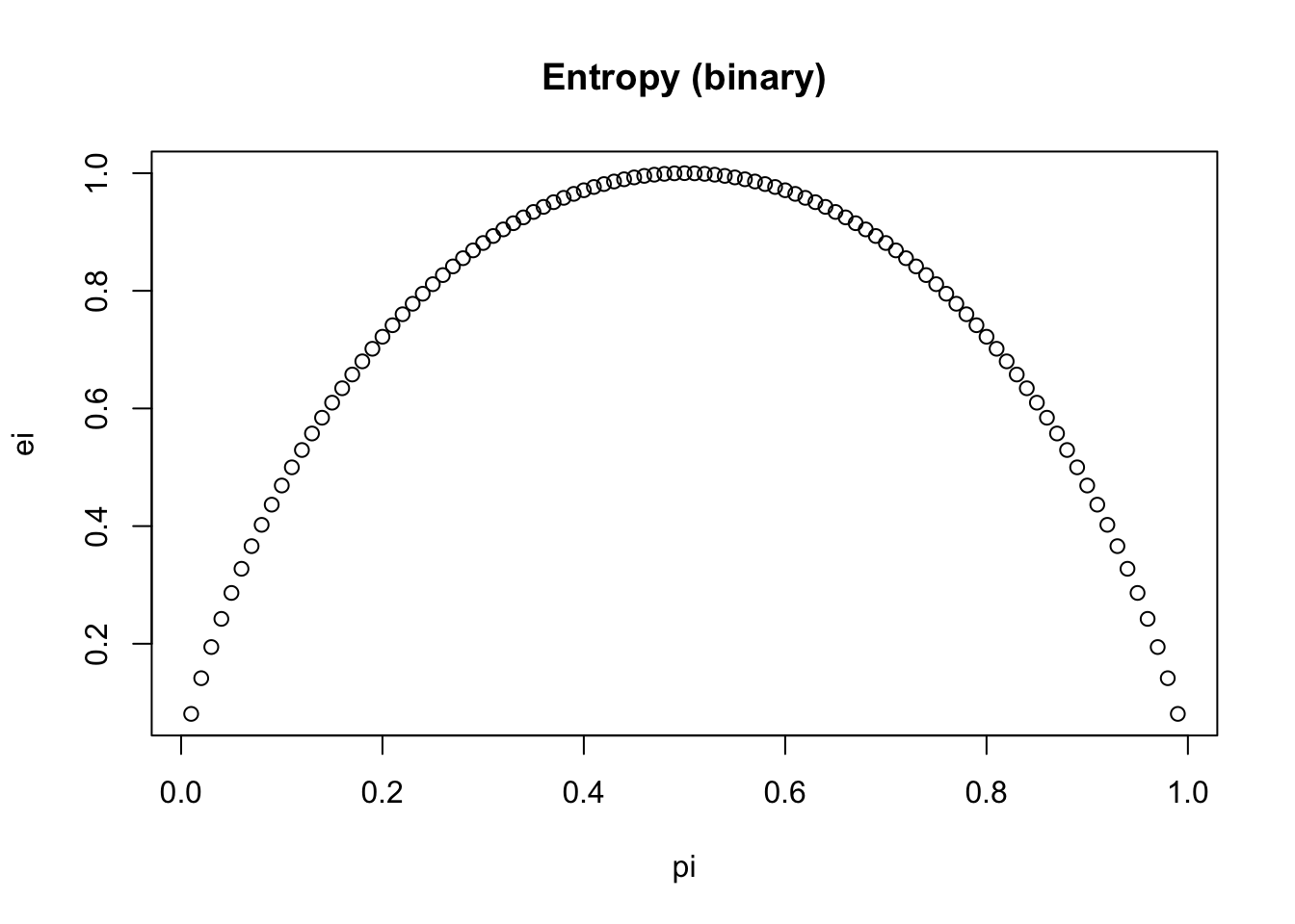
Visualize

pi <- seq(0.01, 0.99, by = 0.01)
ei <- sapply(pi, compute_binary_entropy)
plot(pi, ei, main = 'Entropy (binary)')

In decision tree

• high entropy (close to 1) -> classes are evenly distributed, each having probability of 0.5. High uncertainty, bad split
• low entropy (close to 0) -> low uncertainty, mostly one class, good split

When building a decision tree, we want to reduce entropy and make the nodes purer, rather than having mixed classes in the nodes.

Information gain (IG) is defined as

\[IG = H(parent) - \sum (\frac{N_{child}}{N_{total}} \times H(child))\] We select the split where IG is maximised.

Y	X1	X2
0	no	yes
0	no	no
0	no	yes
1	yes	yes

With this example, the original entropy is compute_binary_entropy(1/4) =0.811. Now we try the following two splits:

X1

• left branch no -> 3 zeros; right branch yes -> 1 yes
• entropy for left: 0; entropy for right: 0 (since both are pure)
• IG: 0.811 - 0 = 0.811

X2

• left branch no -> 1 zero; right branch yes -> 2 zeros, 1 yes
• entropy for left: 0; entropy for right: compute_binary_entropy(1/3) = 0.918
• compute weighted sum at the split

ws <- 1/4 * 0 + 3/4 * compute_binary_entropy(1/3)
ws

[1] 0.6887219

Information gain for this case is 0.811 - 0.689 = 0.122

Now compare the IG at X1 and X2, it’s clear that X1 is producing a purer node, and hence is a better split.

Cross entropy in classification models

Cross entropy measures the differences between true labels and predicted probabilities. For \(p_i\), \(q_i\) being the true class label (0,1) and predicted probability,

\[H(p, q) = -\sum p_i \text{ log } q_i\]

When it is a multi-class problem, \(p_i\) is 1 for the correct class and 0 otherwise.

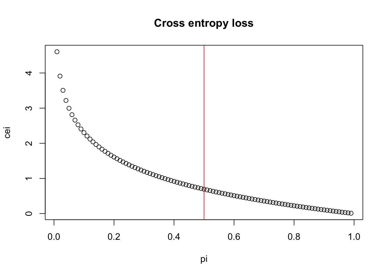
For a data in class 1, the probability is predicted (to be class 1) are 0.9 and 0.2 respectively by two models. By computing the cross entropy we can see that the one with high probability of being in class 1 (correct) produces lower entropy (0.105) rather than higher (1.60).

compute_cross_entropy <- function(p, q){
  e = -1*(p*log(q) + (1-p)*log(1-q))
  return(e)
}
compute_cross_entropy(p=1, q = 0.9) 

[1] 0.1053605

compute_cross_entropy(p=1, q = 0.2) 

[1] 1.609438

pi <- seq(0.01, 0.99, by = 0.01)
cei <- c()
for (i in 1:length(pi)){cei[i] <- compute_cross_entropy(p=1, q=pi[i])}
plot(pi, cei, main = 'Cross entropy loss')
abline(v = 0.5, col = 'red')