Intervals

Confidence, credible and prediction intervals

Key difference: confidence and credible intervals: about the (unknown) parameter; prediction interval: about individual (unseen) observations.

Confidence vs credible interval

Confidence interval (frequentist), about the unknown but fixed parameter. That means, the parameter is not treated as a random variable so does not have a probability distribution. CI is random because it is based on your sample.

Credible interval (Bayesian), associated with posterior distribution of the parameter. The parameter is treated as a random variable hence has a probability distribution.

Prediction intereval

In a regression model, you might want to know both confidence and prediction intervals.

• CI for mean value of \(y\) when \(x =0\), the mean response (e.g. growth of GDP), this is a parameter, an average
• PI for \(y\) when \(x=0\), this is an individual observation.

In simple linear regression

Standard deviation for linear predictor \(\alpha + \beta x\) is

\(\hat{\sigma}_{linpred} = \hat{\sigma} \sqrt{\frac{1}{n} + \frac{(x_{new} - \bar{x})^2}{\sum(x_i - \bar{x})}}\)

Confidence interval

\(\hat{y_{new}} \pm t_{1-\frac{\alpha}{2}, n-2} \times \sqrt{\hat{\sigma}^2 (\frac{1}{n} + \frac{(x_{new} - \bar{x})^2}{\sum(x_i - \bar{x})^2})}\)

Standard deviation for the predicted value \(\alpha + \beta x + \epsilon\) is

\(\hat{\sigma}_{prediction} = \hat{\sigma} \sqrt{1 + \frac{1}{n} + \frac{(x_{new} - \bar{x})^2}{\sum(x_i - \bar{x})}}\)

Prediction interval (frequentist)

\(\hat{y_{new}} \pm t_{1-\frac{\alpha}{2}, n-2} \times \sqrt{\hat{\sigma}^2 (1 + \frac{1}{n} + \frac{(x_{new} - \bar{x})^2}{\sum(x_i - \bar{x})^2})}\)

Posterior predictive distribution

Difference between posterior distribution and posterior predictive distribution PPD

• posterior dist \(p(\theta|x) = c \times p(x|\theta)p(\theta)\), depends on the parameter \(\theta\)
• PPD does not depend on \(\theta\) as it is integrated out, for unobserved \(x^*\),

\(p(x^*|x) = \int_{\Theta} c \times p(x^*, \theta|x) d\theta = \int_{\Theta} c \times p(x^*|\theta)p(\theta|x) d\theta\)

PD is part of PPD formulation.

• PD explains the unknown parameter (treated as a random variable), conditional on the evidence observed (data).
• PPD is the distribution for the future predicted data based on the data you have already seen.

Example: Mortality

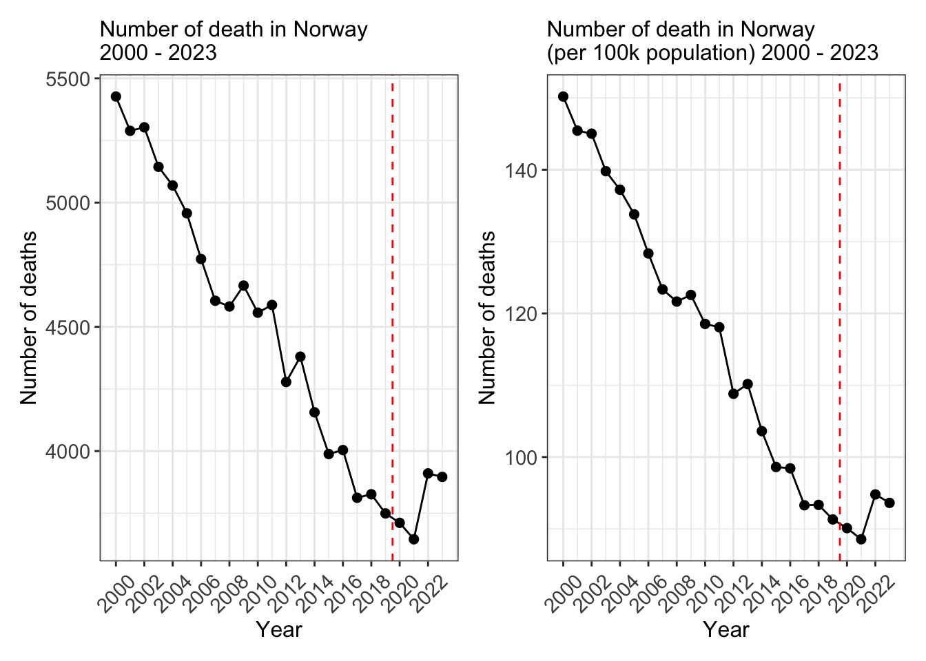
We explore the all-cause mortality counts in Norway between 2000 to 2023. More specifically, we use year 2000-2019 (pre-pandemic years) to fit a simple linear regression model, and predict the expected number of deaths post pandemic (2020-2023). I include both frequentist approach with lm, and Bayesian approach with rstanarm::stan_glm.

The data of mortality example comes from Statistics Norway and is publicly available.

library(ggplot2)
library(patchwork)
library(data.table)
# load data 
mortality <- readRDS("data/mortality_2000_2023.rds")

# select only total age group
d <- mortality[age == '000_059']
d

     year deaths_n     age pop_jan1_n deaths_vs_pop_per_100k
    <num>    <num>  <char>      <num>                  <num>
 1:  2000     5427 000_059    3613275              150.19615
 2:  2001     5289 000_059    3636329              145.44889
 3:  2002     5303 000_059    3656613              145.02492
 4:  2003     5144 000_059    3679479              139.80240
 5:  2004     5069 000_059    3694134              137.21755
 6:  2005     4957 000_059    3705027              133.79120
 7:  2006     4773 000_059    3718828              128.34689
 8:  2007     4605 000_059    3733477              123.34347
 9:  2008     4582 000_059    3766509              121.65111
10:  2009     4666 000_059    3806779              122.57081
11:  2010     4557 000_059    3844344              118.53778
12:  2011     4588 000_059    3885654              118.07536
13:  2012     4278 000_059    3931709              108.80765
14:  2013     4380 000_059    3976015              110.16055
15:  2014     4156 000_059    4011213              103.60956
16:  2015     3988 000_059    4044006               98.61509
17:  2016     4004 000_059    4067801               98.43156
18:  2017     3812 000_059    4086278               93.28783
19:  2018     3826 000_059    4099015               93.33950
20:  2019     3749 000_059    4105628               91.31368
21:  2020     3711 000_059    4118541               90.10472
22:  2021     3645 000_059    4115975               88.55739
23:  2022     3910 000_059    4124531               94.79866
24:  2023     3896 000_059    4161429               93.62169
     year deaths_n     age pop_jan1_n deaths_vs_pop_per_100k

Explore the data

q1 <- ggplot(d, aes(x = year, y = deaths_n, group))
q1 <- q1 + geom_line()
q1 <- q1 + geom_point(size = 2)
q1 <- q1 + geom_vline(xintercept = 2019.5, color = "red", lty = 2)
q1 <- q1 + theme_bw()
q1 <- q1 + scale_x_continuous(breaks = seq(2000, 2023, 2))
q1 <- q1 + labs(
  x = 'Year', 
  y = 'Number of deaths', 
  title = 'Number of death in Norway \n2000 - 2023'
)
q1 <- q1 + theme(
  axis.text = element_text(size = 11),
  axis.title = element_text(size = 12), 
  plot.title = element_text(size = 12), 
  axis.text.x = element_text(angle = 45, vjust = 0.5) 
)
# q1

# per 100k
q2 <- ggplot(d, aes(x = year, y = deaths_vs_pop_per_100k))
q2 <- q2 + geom_line()
q2 <- q2 + geom_point(size = 2)
q2 <- q2 + geom_vline(xintercept = 2019.5, color = "red", lty = 2)
q2 <- q2 + theme_bw()
q2 <- q2 + scale_x_continuous(breaks = seq(2000, 2023, 2))
q2 <- q2 + labs(
  x = 'Year', 
  y = 'Number of deaths', 
  title = 'Number of death in Norway \n(per 100k population) 2000 - 2023'
)
q2 <- q2 + theme(
  axis.text = element_text(size = 11),
  axis.title = element_text(size = 12), 
  plot.title = element_text(size = 12), 
  axis.text.x = element_text(angle = 45, vjust = 0.5) 
)
# plot side by side
q1 + q2

Model mortality using 2000-2019 data

# take pre 2019 data
dt <- d[year <= 2019, .(year, deaths_vs_pop_per_100k)]

# prediction 
dnew <- data.frame(year = c(2020, 2021, 2022, 2023))

Linear regression with lm

m_linear <- lm(deaths_vs_pop_per_100k ~ year, 
               data = dt)

# summary(m_linear)

# produce two intervals
pred_freq_pi <- predict(m_linear, newdata = dnew, interval = 'prediction')
pred_freq_ci <- predict(m_linear, newdata = dnew, interval = 'confidence')

Verify from formula

# verify with formula
n <- nrow(dt)

# option 1
fitted_val <- m_linear$fitted.values
mse <- sum((dt$deaths_vs_pop_per_100k - fitted_val)^2)/(n-2)
mse

[1] 4.383279

# option 2
sum((m_linear$residuals)^2)/(n-2)

[1] 4.383279

# option 3
summary(m_linear)$sigma^2

[1] 4.383279

# option 4
dvmisc::get_mse(m_linear)

[1] 4.383279

# t-val
tval <- qt(p=0.975, df=n-2)
mean_x <- mean(dt$year)

# sum(xi - xbar)^2
ssx <- sum((dt$year - mean_x)^2)

sd_confint <- sqrt(mse * (1/20+ ((dnew$year - mean_x)^2)/ssx))
sd_predint <- sqrt(mse * (1 + 1/20+ ((dnew$year - mean_x)^2)/ssx))


# point prediction
b0 <- coef(m_linear)[1]
b <- coef(m_linear)[2]
prednew <- b0 + b*dnew$year
prednew

[1] 85.68773 82.50765 79.32757 76.14749

# prediction interval
predint_linear <- data.frame(fit = prednew, 
                             lwr = prednew - tval*sd_predint, 
                             upr = prednew + tval*sd_predint)

predint_linear

       fit      lwr      upr
1 85.68773 80.83777 90.53770
2 82.50765 77.59214 87.42316
3 79.32757 74.34154 84.31360
4 76.14749 71.08617 81.20880

pred_freq_pi # compare with result from lm

       fit      lwr      upr
1 85.68773 80.83777 90.53770
2 82.50765 77.59214 87.42316
3 79.32757 74.34154 84.31360
4 76.14749 71.08617 81.20880

# confidence interval
confint_linear <- data.frame(fit = prednew, 
                             lwr = prednew - tval*sd_confint, 
                             upr = prednew + tval*sd_confint)

confint_linear

       fit      lwr      upr
1 85.68773 83.64447 87.73100
2 82.50765 80.31334 84.70196
3 79.32757 76.97954 81.67560
4 76.14749 73.64355 78.65142

pred_freq_ci # compare with result from lm

       fit      lwr      upr
1 85.68773 83.64447 87.73100
2 82.50765 80.31334 84.70196
3 79.32757 76.97954 81.67560
4 76.14749 73.64355 78.65142

Linear regression with rstanarm

m_bayes <- rstanarm::stan_glm(
  deaths_vs_pop_per_100k ~ year, 
  data = dt, 
  family = gaussian,
  iter = 2000,
  chains = 8,
  refresh = 0
)

m_bayes 

stan_glm
 family:       gaussian [identity]
 formula:      deaths_vs_pop_per_100k ~ year
 observations: 20
 predictors:   2
------
            Median MAD_SD
(Intercept) 6508.1  177.4
year          -3.2    0.1

Auxiliary parameter(s):
      Median MAD_SD
sigma 2.2    0.4   

------
* For help interpreting the printed output see ?print.stanreg
* For info on the priors used see ?prior_summary.stanreg

sims <- as.matrix(m_bayes)
median <- apply(sims, 2, median)
median
mad_sd <- apply(sims, 2, mad) 
# median absolute deviation (similar to sd)
mad_sd

Credible interval

# credible interval about the fit
cred <- rstanarm::posterior_interval(m_bayes, prob = 0.95)
cred

                   2.5%       97.5%
(Intercept) 6152.417192 6860.192409
year          -3.354741   -3.002696
sigma          1.627436    3.189029

# equivalent to
sims <- as.matrix(m_bayes)
apply(sims, 2, quantile, probs = c(0.025, 0.5, 0.975))

       parameters
        (Intercept)      year    sigma
  2.5%     6152.417 -3.354741 1.627436
  50%      6508.056 -3.179352 2.189433
  97.5%    6860.192 -3.002696 3.189029

Point prediction

# point predict
# uses median from the posterior sim
y_point_pred <- predict(m_bayes, newdata = dnew)
y_point_pred

       1        2        3        4 
85.69576 82.51670 79.33763 76.15857 

a_hat <- coef(m_bayes)[1] # median
b_hat <- coef(m_bayes)[2] # median
a_hat + b_hat*dnew$year

[1] 85.76544 82.58609 79.40673 76.22738

Uncertainty of linear predictor

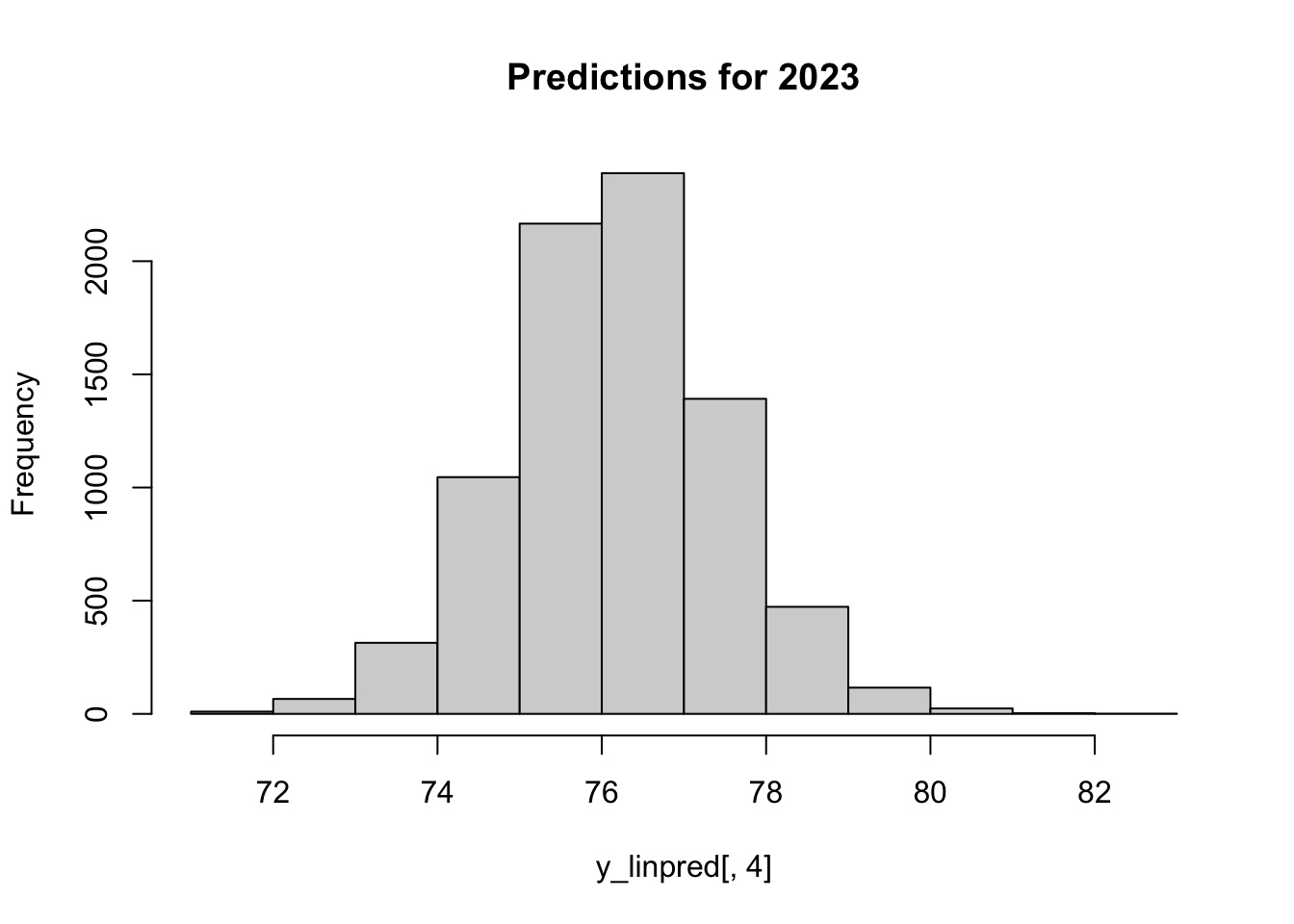
The uncertainty of linear predictor, \(a + bx\) is propagated through the uncertainty in \(a\) and \(b\), respectively. For now the error term is not included.

rstanarm::posterior_linpred is equivalent to using each pairs of \(a, b\) from the posterior distribution to compute the point predictions.

# linear predictor with uncertainty via a's and b's
y_linpred <- rstanarm::posterior_linpred(m_bayes, newdata = dnew)
head(y_linpred)

          
iterations        1        2        3        4
      [1,] 85.08325 81.84939 78.61552 75.38165
      [2,] 85.88709 82.75122 79.61535 76.47947
      [3,] 84.95982 81.79409 78.62837 75.46264
      [4,] 85.53266 82.25730 78.98193 75.70656
      [5,] 84.97415 81.68506 78.39597 75.10688
      [6,] 84.78472 81.47082 78.15692 74.84302

# focus on one year: 2023
hist(y_linpred[, 4], main = 'Predictions for 2023')

head(y_linpred[, 4])

[1] 75.38165 76.47947 75.46264 75.70656 75.10688 74.84302

y_linpred_byhand <- sims[,1] + dnew$year[4] * sims[,2]
y_linpred_byhand[1:6]

[1] 75.38165 76.47947 75.46264 75.70656 75.10688 74.84302

Posterior predictive distribution

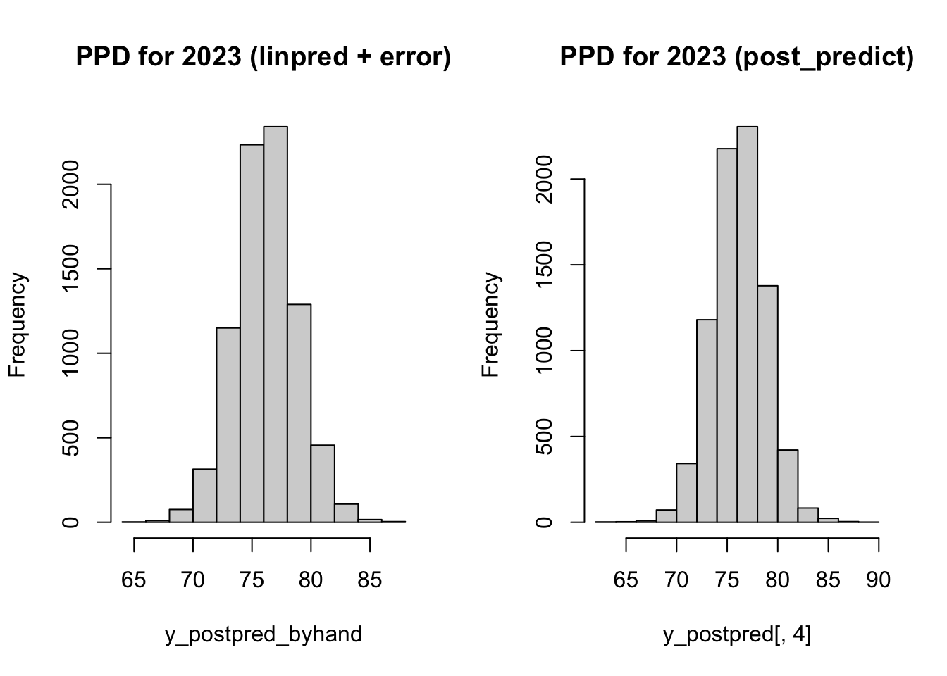
With PPD, include the additional uncertainty in \(\sigma\). This is equivalent to using the linear predictor from above, plus a random draw from rnorm(1, 0, sigma).

Due to randomness in the error, we can not get the exact same results. But they should be close enough.

# posterior predictive dist (with sigma)
y_postpred <- rstanarm::posterior_predict(m_bayes, newdata = dnew)
head(y_postpred)

            1        2        3        4
[1,] 82.68850 84.34282 78.83013 77.50019
[2,] 85.33044 85.78202 79.12413 76.06252
[3,] 85.29410 83.10030 80.19248 76.12616
[4,] 88.07453 76.55464 80.95563 67.89540
[5,] 82.71118 81.78970 75.92396 76.66999
[6,] 82.54895 84.17229 85.07779 76.85435

# by hand
# focus on one year: 2023
n_sim <- nrow(sims)
y_postpred_byhand <- y_linpred_byhand + rnorm(n_sim, 0, sims[,3])
par(mfrow = c(1,2))
hist(y_postpred_byhand, main = 'PPD for 2023 (linpred + error)')
hist(y_postpred[,4], main = 'PPD for 2023 (post_predict)')

y_postpred[,4] |> summary()

   Min. 1st Qu.  Median    Mean 3rd Qu.    Max. 
  63.20   74.45   76.16   76.17   77.91   88.14 

y_postpred_byhand |> summary()

   Min. 1st Qu.  Median    Mean 3rd Qu.    Max. 
  65.15   74.50   76.16   76.20   77.87   87.60 

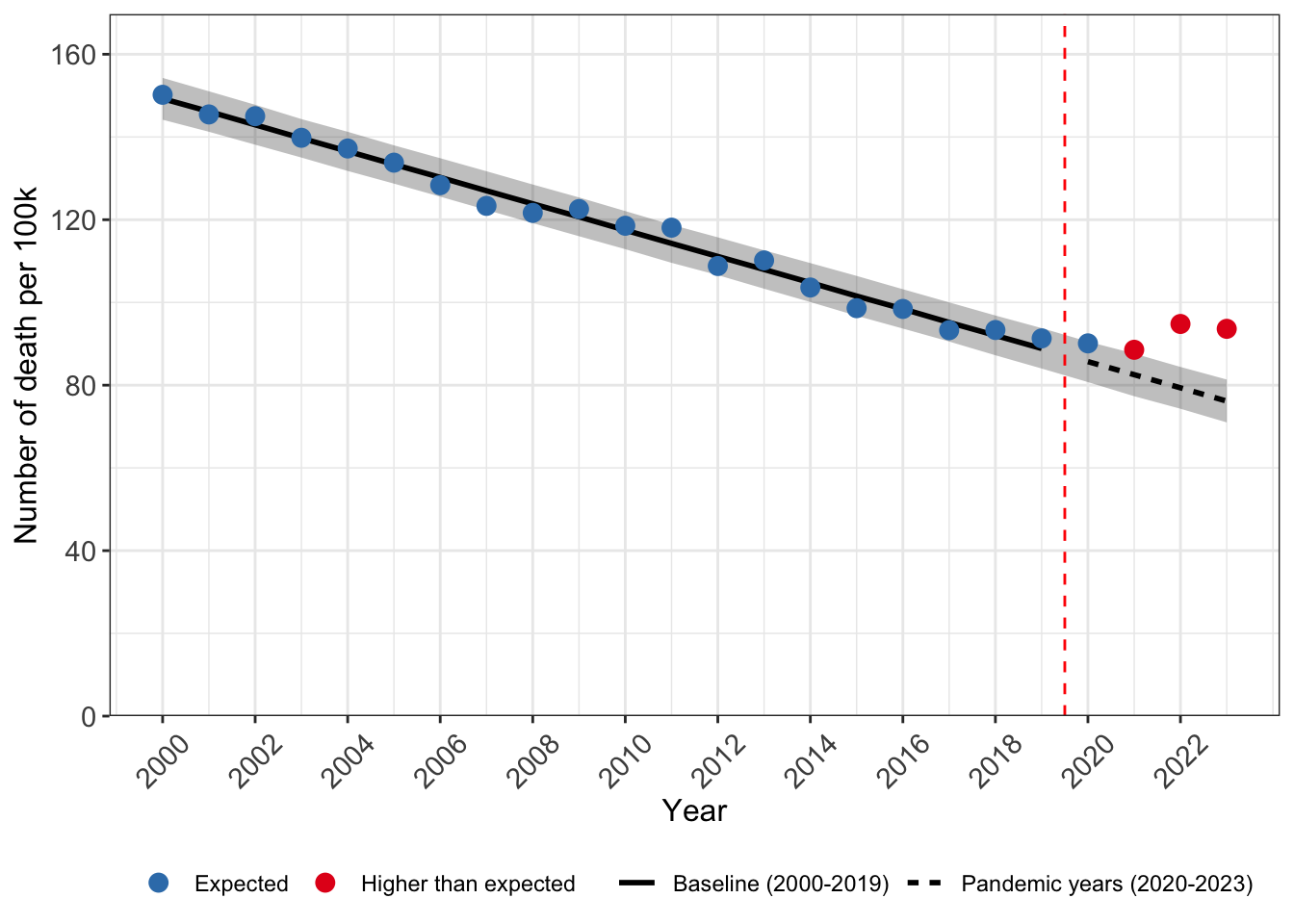
Prediction for 2020-2023 mortality

Here we choose to use rstanarm::posterior_predict().

pred_all <- rstanarm::posterior_predict(m_bayes, d)

pred_all_quantile <- apply(pred_all, 2, quantile, 
                    probs = c(0.025, 0.5, 0.975)) |> 
  t()  |> 
  as.data.frame()
pred_all_quantile[21:24,]

       2.5%      50%    97.5%
21 80.74734 85.69239 90.53479
22 77.32815 82.53766 87.64822
23 74.30338 79.36104 84.41148
24 71.00084 76.15183 81.36930

We can compare with the frequentist prediction interval, and we see that they are very close.

predint_linear

       fit      lwr      upr
1 85.68773 80.83777 90.53770
2 82.50765 77.59214 87.42316
3 79.32757 74.34154 84.31360
4 76.14749 71.08617 81.20880

Visualize mortality prediction

pd <- copy(d)
# head(pd)
pd <- cbind(pd, pred_all_quantile)

setnames(pd, old = '2.5%', new = 'exp_death_per100k_025')
setnames(pd, old = '50%', new = 'exp_death_per100k_50')
setnames(pd, old = '97.5%', new = 'exp_death_per100k_975')

# also compute the expected death overall

pd[, exp_death_025 := exp_death_per100k_025 * pop_jan1_n/100000]
pd[, exp_death_50 := exp_death_per100k_50 * pop_jan1_n/100000]
pd[, exp_death_975 := exp_death_per100k_975 * pop_jan1_n/100000]

pd[, alert := fcase(
  deaths_vs_pop_per_100k > exp_death_per100k_975, "Higher than expected",
  default = "Expected"
)]

pd[, type := fcase(
  year <= 2019, paste0("Baseline (2000-2019)"),
  default = "Pandemic years (2020-2023)"
)]


# make plot
q <- ggplot(pd, aes(x = year))
q <- q + geom_ribbon(mapping = aes(ymin = exp_death_per100k_025, 
                                   ymax = exp_death_per100k_975), 
                     alpha = 0.3)
q <- q + geom_line(mapping = aes(y = exp_death_per100k_50, lty = type), linewidth = 1)
q <- q + geom_point(mapping = aes(y = deaths_vs_pop_per_100k, color = alert), size = 3)
q <- q + geom_vline(xintercept = 2019.5, color = "red", lty = 2)
q <- q + expand_limits(y=0)
q <- q + scale_y_continuous("Number of death per 100k", expand = expansion(mult = c(0, 0.1)))
q <- q + scale_x_continuous("Year", breaks = seq(2000, 2023, 2))
q <- q + scale_linetype_discrete(NULL)
q <- q + scale_color_brewer(NULL, palette = "Set1", direction = -1)
q <- q + theme_bw()
q <- q + theme(
  axis.text = element_text(size = 11),
  axis.title = element_text(size = 12), 
  plot.title = element_text(size = 15), 
  axis.text.x = element_text(angle = 45, vjust = 0.5) 
)
q <- q + theme(legend.position = "bottom", legend.direction = "horizontal")
q <- q + theme(legend.box = "horizontal", legend.margin = margin(2, 2, 2, 2))
q

Reference

• A very good decomposition of prediction interval in linear regression: Post by Bryan Shalloway
• Blog by Professor Rob Hyndman on difference between prediction intervals and confidence intervals
• The data of mortality example comes from Statistics Norway and is publicly available.